Implementing kernalized regression from scratch in python
Originally published on medium.com on 10. March 2021.
Okay, there are already plenty of articles describing linear regression but I have not seen much on kernelized regression. Well the fact that you are reading this means that you also didn’t find what you were looking for…
For completeness we will get started with ordinary linear regression.
Ordinary Linear Regression
First we need some data that we can play with. Here we will just create some arbitrary 2 dimensional samples.
import numpy as np
import matplotlib.pyplot as plt

x=np.linspace(2,30,100)
y= 2*(x+15)+np.random.random_sample(x.shape)*5+2
x=x[:,np.newaxis]
show(x,y)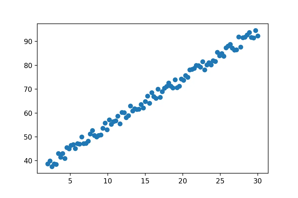
You can think of this data as whatever you want. Here we can clearly see that there is a strong correlation between the two variables. The x-axis could be price of a bus-ticket and y-axis could be the distance traveled, as we would expect a strong correlation there. Youre data likely looks completely different but linear regression works all the same.
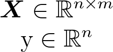
Let’s have a closer look at the data. In our case the data X is just one dimensional but we will take multiple samples so we have n=100 samples each of dimension d=1.
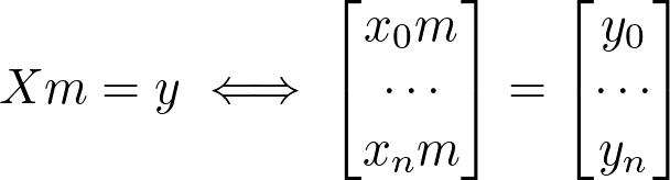
We know the equation of a line is y=mx. We simply let our data X represent the general x and then we just need to solve for m.
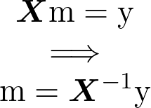
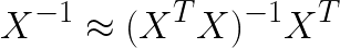
Since we can not invert a matrix that isn’t square we simply make X square by multiplying with its own transpose before inversion. To get the original shape back and by magic of math we multiply by the transpose again and get what’s know as Moore–Penrose inverse.
Okay finally time for more code.
k = np.linalg.inv(np.dot(x.T,x))
m=np.dot(k,np.dot(x.T,y))
show(x,y,0,m)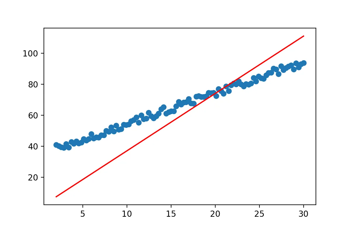
Well we got a line… but it doesn’t really match the data yet. So what went wrong? The line equation that we started with y=mx will always pass through (0,0). No matter what value you pick for m at x=0, y has to be 0. However the regression line we expect from our data does not pass through (0,0). So we have to adjust our line equation so that it’s y-value at x=0 can be fitted by our approach. We all know from school that we can simply add a constant to our line formula to end up with y=mx+b.
How are we going to this with our current equation? Let’s look at what we have so far:
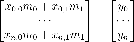
x=np.stack([x[:,0],np.ones(x.shape[0])],axis=1).reshape(-1,2)
k = np.linalg.inv(np.dot(x.T,x))
m=np.dot(k,np.dot(x.T,y))
show(x[:,0],y,m[1],m[0])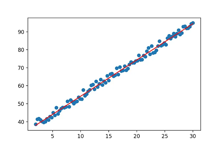
We are not going to discuss the remaining topics in detail. The rest is just to get you started and give you a general idea.
Ridge Regression
Sometimes the pseudo-inverse can run into trouble which can be avoided if we add a small value to our matrix before computing the inverse. This is known as ridge regression.
small_arbitrary_value=0.1
k = np.linalg.inv(np.dot(x.T,x)+small_arbitrary_value*np.eye(x.shape[1]))
m=np.dot(k,np.dot(x.T,y))
show(x[:,0],y,m[1],m[0])
Primal vs Dual Form
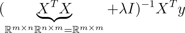
So far we have been implementing the primal form. If we look at the dimensions we notice that the matrix that we have to inverse is a square matrix of the dimension 2. Just like our (extended) samples in X.
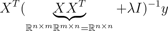
This is known as the dual Form. Notice that the matrix that needs to be inverted is know a square matrix of the dimension n x n. This is much more expensive to compute when we have more samples than dimensions in X. So most of the time we want to avoid this. However it can be useful to derive solutions for classification problems such as SVM so it’s good to have seen this before.
Kernel Regression
We now know how to compute a linear regression. But often data is not linear … we could come up with non linear regression methods. But we just picked up linear regression so let’s see what we can do. If we add a few dimensions to our input data we might be able to a linear regression in the higher dimension(feature space). Or a linear separation as depicted below:
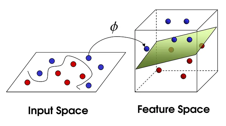
CC BY-SA 4.0Photo by Shehzadex on Wikimedia
What does that transformation look like? Just to give you an idea a simple polynomial mapping could look like this:

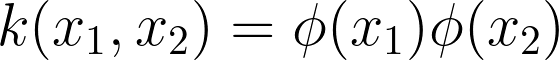

def kernel(x_i,x_j):
    #return np.dot(x_j,x_i) # Linear Kernel, same as not using Kernels at all
    #return np.dot(x_j,x_i)**2 # Polynomial Kernel
    return np.exp(-0.5*np.linalg.norm(x_i-x_j)) # Gaussian Kernel


# let's set up some non linear data
y= np.sin(x[:,0])+x[:,1]
y= x[:,0] + 4*np.sin(x[:,0])+ 4*np.random.rand(x.shape[0])

# We could just call the kernel function every time
# Instead we store the solutions in this matrix
# to save some computations
K=np.zeros((x.shape[0],x.shape[0]))
for i, row in enumerate(K):
    for j, col in enumerate(K.T):
K[i,j]=kernel(x[i,:],x[j,:])Now we just take our by now familiar linear regression and replace all dot products with kernel functions.

a = np.linalg.inv(K+0.1*np.eye(K.shape[0]))
m=np.dot(y,a)

x_pred=np.arange(0,35,0.2)
x_pred=np.stack([x_pred,np.ones(x_pred.shape[0])],axis=1).reshape(-1,2)
y_pred=np.zeros(x_pred.shape[0])
for outer_i, x_p in enumerate(x_pred):
    k = np.zeros(x.shape[0])
    for i, row in enumerate(k):
        k[i]=kernel(x_p,x[i,:])
    y_pred[outer_i]=np.dot(m,k)

show(x[:,0],y,x_2=x_pred[:,0],y_2=y_pred)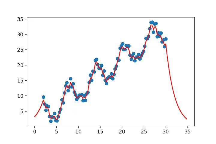
def show(x_sample,y,a=0,b=0, x_2=None,y_2=None):
    if b !=0:
        plt.plot(x_sample,a+b*x_sample , c='red')

    if x_2 is not None:
        plt.plot(x_2,y_2, c='red')
    plt.scatter(x_sample, y)
    plt.show()